Phylogenies are estimated with a greater or lesser degree of uncertainty. It is not easy to take this into account and to assess the effects on the results of mapping shape or other phenotypic traits onto those phylogenies. One approach is to use a range of different trees as an expression of the uncertainty about the tree, for example a set of trees estimated for bootstrapped data (e.g. nucleotide sequences; e.g. Felsenstein 2004).
MorphoJ offers this approach for evaluating the effects of phylogenetic uncertainty on the results of assessment of phylogenetic signals in morphological data (Klingenberg et al. 2012).
Comparative analyses are conducted with some degree of uncertainty about the phylogenetic tree that is used. A way to assess this uncertainty is to conduct a bootstrap analysis that is by repeatedly resampling from the data to simulate the sampling process and estimating the tree from each of the resampled datasets (Felsenstein 1985). The resulting set of bootstrap trees can be used to gauge the statistical uncertainty about the tree: if all the trees are very similar or even identical, there is little or no uncertainty, but if they differ much from each other, there is much uncertainty and any phylogenetic inferences need to be interpreted cautiously. Other statistical approaches than the bootstrap, e.g. in a Bayesian perspective, also can represent the uncertainty about a phylogenetic tree by a set of trees that are in some way considered to be "possible estimates" of the tree.
The resulting set of trees can in turn be used to examine the consequences of this uncertainty on the results of mapping morphometric data onto the phylogenetic tree (Klingenberg et al. 2012). Specifically, the tree lengths under squared-change parsimony and the P-value for the permutation test of phylogenetic signal (Klingenberg & Gidaszewski 2010) are computed for all trees in the set; the distribution of these statistics, relative to their values for the preferred phylogenetic tree, can be used to assess the effects of phylogenetic uncertainty (Klingenberg et al. 2012). The variation of estimated tree lengths for the different trees, with the same morphometric data mapped onto each of the trees, can be interpreted as a measure of uncertainty about the tree length. Likewise, the variation of the P-value for the permutation test can be interpreted as a measure of how phylogenetic uncertainty affects the test. If the test is significant for the preferred tree as well as all resampled trees, there is no effects of phylogenetic uncertainty on the test of phylogenetic signal. Likewise, if the preferred tree and the resampled trees all yield non-significant permutation tests, phylogenetic uncertainty can be ruled out as an explanation for the non-significant result. If the resampled trees yield a range of P-values that include significant as well as non-significant ones, the results of the test should be interpreted cautiously because phylogenetic uncertainty has a marked effect.
The tree lengths and permutation tests are computed in the same way as in the procedure Map Onto Phylogeny, i.e. with squared-change parsimony (Maddison 1991) and the permutation test for phylogenetic signal as described by Klingenberg & Gidaszewski (2010).
The study by Klingenberg et al. (2012) is an example in which the method is applied.
Before the analysis can start, a phylogeny tree set must be imported using Import Phylogeny Tree Set in the File menu.
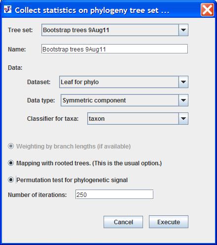
To start the analysis, select Collect Statistics on Tree Set in the Comparison menu. If the dataset or the tree set to be used in the analysis are selected in the Project Tree before invoking the command, they will be pre-selected in the dialog box. A dialog box like the following will appear:
The first item in this dialog box contains is a drop-down menu for choosing the Tree Set to be used in the analysis.
Below it is a text field for entering a name for the analysis ("Bootstrap trees 9Aug11" in the screen shot above). The analysis appear in the Project Tree as another Tree Set, so it is a good idea to modify the name (by default, it is the same as the name of the Tree Set selected for the analysis).
The next items concern the choice of data. There are three drop-down menus: one for the dataset (named "Leaf for phylo" in the example above), one for the data type and one for the classifier that contains the taxon names (exactly as they are in the Tree Set; note especially the convention that underscores in NEXUS files are changed into spaces -- see Import Phylogeny Files for more details).
The remaining choices concern the options for the analysis itself.
Depending on whether the phylogenies have associated branch lengths or not, the button Weighting by branch lengths is activated or not. This option makes the choice between weighted and unweighted squared-change parsimony as the mapping method (Maddison 1991).
The button Mapping with rooted trees is to choose whether rooted (if the button is selected) or unrooted (if it is unselected) trees are to be used. The usual option is to use rooted trees (for squared-change parsimony, this choice does make a difference, albeit usually a fairly small one; Maddison 1991, Klingenberg & Gidaszewski 2010).
Finally, there is a button for including the Permutation test for phylogenetic signal (Klingenberg & Gidaszewski 2010). If this option is chosen, a permutation test will be conducted for each of the trees in the Tree Set. Note that this can take a considerable amount of time if there are many trees in the set. Therefore, the Number of iterations for each tree should be chosen with care (the default is set to 250 iterations for each tree).
The Execute button starts the analysis (note that the permutation tests can take some time). Clicking the Cancel button aborts the procedure and closes the dialog box.
The graphical output consists of two or three components: the phylogenetic trees in the Tree Set, the distribution of tree lengths and, if the option for the permutation test is selected, the distribution of P-values of the permutation tests for all trees.
The first tab contains diagrams of the trees in the Tree Set. By default, the first tree in the Tree set appears in the tab. To select another tree, invoke the pop-up menu of the graph and use the first entry, Select the Tree to Display. This will bring up a dialog box where you can select any tree from the Tree Set.
The second tab is a histogram that shows the distribution of tree lengths for the trees in the Tree Set and the data chosen for the analysis. The reference for comparison is the tree length obtained when the preferred phylogeny is used with the procedure Map Onto Phylogeny.
If the option for the permutation test was selected, the distribution of P-values for the permutation tests on all trees is also shown as a histogram.
The output contains a summary of the dataset, the Tree Set (including the number of trees), the variables used in the analysis and, if a permutation test for a phylogenetic signal was done, the number of permutations.
The output further provides the minimum and maximum, as well as the quantiles for 2.5%, 5%, 10%, 50% (median), 90%, 95%, 97.5% for the tree lengths and, if the option for permutation tests was selected, for the P-values of the tests for phylogenetic signal.
Felsenstein, J. 1985. Confidence limits on phylogenies: an approach using the bootstrap. Evolution 39:783–791.
Klingenberg, C. P., and N. A. Gidaszewski. 2010. Testing and quantifying phylogenetic signals and homoplasy in morphometric data. Systematic Biology 59:245–261.
Klingenberg, C. P., S. Duttke, S. Whelan, and M. Kim. 2012. Developmental plasticity, morphological variation and evolvability: a multilevel analysis of morphometric integration in the shape of compound leaves. Journal of Evolutionary Biology 25:115–129.
Maddison, W. P. 1991. Squared-change parsimony reconstructions of ancestral states for continuous-valued characters on a phylogenetic tree. Systematic Zoology 40:304–314.