
Regression is a technique for predicting the values of one or more dependent variables from the values of one or more independent variables. Therefore, there is an inherent asymmetry between the dependent variables (to be predicted) and the independent variables (predictors) that distinguishes regression from other techniques of analyzing covariance between sets of different variables, such as partial least squares.
The implementation of regression in MorphoJ is flexible in that there can be both multiple independent variables (multiple regression) and multiple dependent variables (multivariate regression). The dependent variables must all be from one dataset, but the independent datasets can be from one or more datasets, provided that they are linked to the dataset containing the dependent variables.
Regression can also be used to remove the influence of other variables, for instance, for size correction of shape data (e.g. Klingenberg 2016). For this purpose, each regression analysis in MorphoJ produces a new dataset containing the residuals from the regression, which can be used in further analyses.
Regression is used for a variety of purposes in geometric morphometrics. This great flexibility corresponds to the simplicity of the model that underlies it; it all depends on the kinds of data used as dependent and independent variables.
MorphoJ provides two general options for regressions: the usual type of regression in a single sample and pooled within-group regression (related to analysis of covariance; e.g. Klingenberg 2016).
Here I briefly outline the use of regresssion residuals as a means of correcting for the effects of external factors such as size, environmental quality and the likes. I will use size correction as the example throughout this section. But the correction for other factors proceeds in an analogous manner (just substitute your external factor or factors for size as the independent variable).
The key idea is that regression separates the component of variation in the dependent variables that is predicted by the independent variable from the residual component of variation, which is uncorrelated with the independent variables. In the diagram below, this decomposition is shown for a single data point (black dot). Its deviation from the sample average (hollow dot) in the direction of the shape variable (vertical; the dependent variable) is divided into a predicted and a residual component. The predicted compoent can be computed from the slope of the regression line (bold oblique line) and the deviation of the data point from the mean in the direction of size (horizontal; the independent variable). The residual is the difference of the total shape deviation of the data point from the mean and the predicted component.
If we remove the predicted component from the analysis and focus exclusively on the residuals, this new variable is uncorrelated with the independent variable. This is an effective way, for example, to remove the effect of size on shape. Using the residuals from a regression of shape on size for further analyses is therefore a method of size correction for the shape data.
If we are considering more than one group at a time and if the regression slopes in the groups are the same, we can perform a pooled within-group regression (e.g. Klingenberg 2016). This method uses the regression slopes within samples to separate the predicted and residual components of variation in the dependent variables.
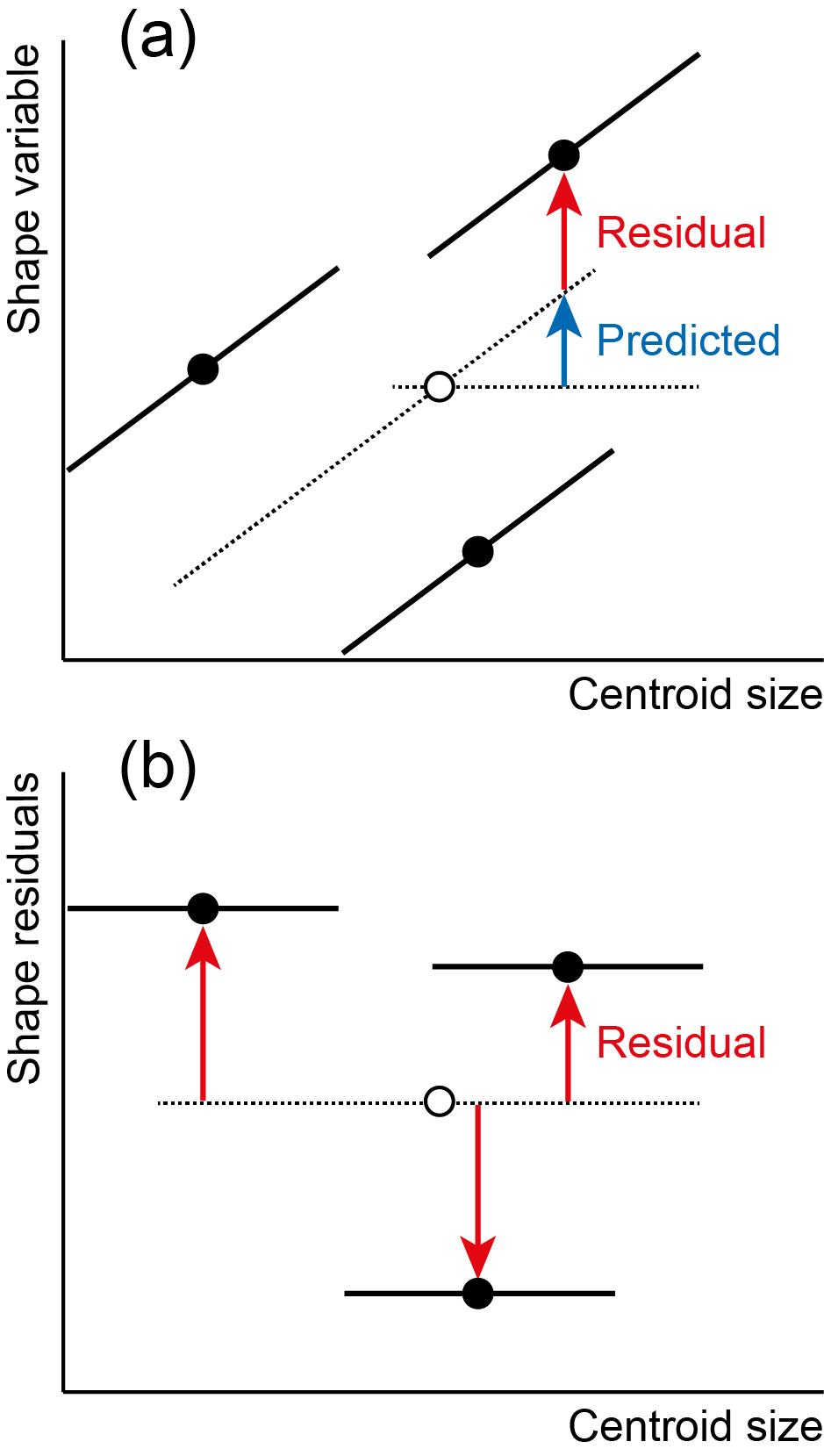
Note that there is not just a separation of predicted and residual deviations for individual data points, but now also for the means of the subsamples corresponding to the different groups. The correct decomposition of the group differences is obtained if predicted values and residuals are computed from the grand mean to each of the group means (Klingenberg 2016).
Warning: Versions of MorphoJ up to version 1.01c contain an error in the computation of residuals for pooled within-group regression. If you use this method, make sure you use version 1.02a or a more recent version.
Regression is often used to correct for the effects of size on shape. If the allometric relationship between size and shape can be represented with sufficient accuracy by a linear regression of shape on size, the residuals from that regression are shape values from which the effects of size have been removed (e.g. Klingenberg 2016).
Size correction in geometric morphometrics usually uses a regression of shape on centroid size, or sometimes the regression of shape on log-transformed centroid size. The choice between these two options should be based on which one of these size measures produces the better linear relationship. In many biological datasets, there is no big difference between them because the range of size is relatively small (particularly if studies include only adult organisms). In ontogenetic studies including very early stages or very lare size ranges, shape change is often concentrated disproportionately in the early stages and small sizes. In this situation, size correction using log-transformed centroid size will usually perform better.
If the dataset contains multiple groups, the question arises whether this group structure should be considered for size correction. In other words, the question is whether the correction should be specifically for the within-group allometric relationship or for the total allometry. This question does matter because the within- and between-group allometries cannot be expected to coincide in general.
If group structure is to be considered, size correction should be based on pooled within-group regression. This results in a reduction of shape variation within groups, which sometimes can lead to a substantial increase in the separation of groups.
These methods are not restricted to size, but can also be used for correcting shape data for the influence of extrinsic factors such as age or environmental quality, which otherwise might introduce heterogeneity that might interfere with the analysis. Such variables can be included as covariates.
For each independent variable, MorphoJ computes a vector of regression scores for all the observations in the sample, mainly as a means for visualizing the relationship (Drake and Klingenberg 2008).
Consider the regression equation y = xB + e, where y is the random vector of dependent variables (usually shape), x is the random vector of independent variables, B is the matrix of regression coefficients, and e is the random vector of error effects. A new variable si can be defined as si = ybiT(biTbi)-0.5, where bi is the regression vector for the i-th independent variable (xi) and shape. This is simply a projection of the vector y onto the direction of the regression vector bi. In the context of a regession of a shape vector on one or more independent variables, the regression score si can be interpreted as the shape variable that is most strongly associated with the i-th independent variable.
The permutation test associated with the regression analysis uses the null hypothesis of complete independence between the dependent and independent variables. It simulates this null hypothesis by randomly reassigning observations for the dependent variable(s) to observations for the independent variable(s).
The test statistic is the sum of squares predicted by the regression, summed across all the dependent variables. If the dependent variables are shape variables, this is the Procrustes sum of squares, and the test is equivalent to a test using Goodall's F statistic.
If there are multiple dependent variables, note that this test statistic, as well as the percentages of predicted and residual variation, only make sense if all the dependent variables are in the same units. This is automatically so if the dependent variables are shape variables (Procrustes coordinates, the symmetric or asymmetry components etc.).
To start a new regression analysis, select Regression... in the Covariation menu. The following dialog box will then appear:
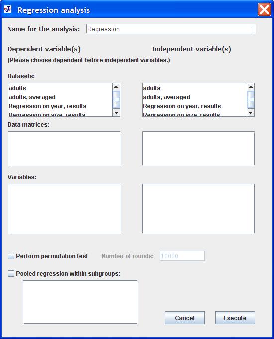
The text field at the top, with the default entry "Regression", is for entering the name of the analysis as it will appear in the project tree.
The subsequent elements are for selecting the dependent and independent variables. Select the dependent variables (left column) before the independent variables (right column), because changes of the selections for the dependent variables may affect the options available for the independent variables.
In each of the two columns, the top window is for selecting the dataset or datasets. For the dependent variables, only one dataset at a time can be selected. In response to this selection, the list of datasets for the independent variables will show only those datasets that are linked to the dataset selected for the dependent variables. For the independent variables, more than one dataset can be selected. The second window in each column shows the data matrices in the datasets selected in the respective column. The third window in each column lists the variables in the selected data matrices. For many data types, for instance Procrustes coordinates, all variables need to be considered jointly and only a single entry thererfore appears for all variables together. For other data types, such as covariates, all variables are listed and can be selected individually.
Below the lists of variables, there is a check box for selecting whether a permutation test is to be performed. This test is against the null hypothesis of independence between the dependent and independent variables. If the check box is selected, the text field for entering the number of permutation runs is activated (with a default value of 10,000 rounds).
The bottom element is for selecting a pooled within-group regression. This type of regression is suitable, for instance, for removing the effect of within-group variation of a variable such as size, age or environmental factors before comparisons between groups. The analysis is performing a regression using the deviations of the dependent and independent variables from the respective group means (the group means are added back to the residuals and predicted values in the output dataset). If the check box 'Pooled regression within subgroups' is selected, the list can be used so select one or more of the classifiers in the dataset of the dependent variables as the grouping criterion.
The graphical output from a regression analysis contains one or two panels:
If shape is used for the dependent variables, there is a graph with the shape changes corresponding to the regression vector for each independent variable (to change the independent variable, use "Change Variable to Display ..." in the pop-up menu of the graph). The starting shape in this graph is the mean shape. By default, graph shows the shape change for an increase of the independent variable by one unit. The magnitude and the direction of the shape change can be changed by altering the magnitude and the sign of the scale factor. The default setting for the scale factor in this graph is 1.0 (an increase of the independent variable by one unit); this can be changed by using the popup menu to alter the scale factor (you may want to check the range of the independent variable in the Score scatter plot and set the scale factor accordingly).
In any case, there is a scatter plot of the regression scores (see above) against the corresponding independent variable. If more than one independent variable is used, there is a plot for each of them (to change the variable, use "Choose Independent Variable ..." in the pop-up menu of the graph).
For pooled within-group regression analyses, there is an extra scatter plot of group-centered scores. This plot differs from the preceding plot of regression scores by having average scores of 0.0 as well as average values of 0.0 for the corresponding independent variable in each of the groups. This plot visualizes the relationship that is used to compute the pooled within-group regression.
The text output first provides information about the dependent and independent variables and the sample size. If a pooled within-group regression is used, the sample sizes of the groups are also indicated.
Next, the regression coefficients are listed.
To indicate the relative amount of variation for which the regression accounts, the output provides the total, predicted and residual sums of squares. If shape is used for the independent variables, these sums of squares are in units of squared Procrustes distance. The output also provides the proportion of variation for which the regression accounts as a percentage of the total variation.
If the option for pooled within-group regression is selected, these values are computed from the pooled within-group variation.
Two caveats are in order concerning these statistics. First, the proportion of total variation for which the regression accounts is meant as a general indicator of the magnitude of the regression effects, but it is not a formal statistic for evaluating the regression. It is an informal analogue to the R-squared from bivariate or multiple regression with a single dependent variable (in some sense, collapsing the information from all dimensions into a single index goes against the spirit of multivariate analysis). In particular, if some aspects of shape respond to a factor and others do not, a regression may be both biologically and statistically significant, even though only little of the total shape variation may be accounted for.
Second, if the dependent variables are not shape, the various sums of squares are only meaningful if all dependent variables are in the same units.
If a permutation test has been requested, the output also provides the number of permutation rounds and the P-value.
The regression analysis generates a new dataset that contains the residuals and predicted values as well as the regression scores for every observation in the analysis. This dataset can be used for further analyses. For instance, using the residuals from a regression of shape on centroid size is a method to correct for the effects of allometry.
Drake, A. G., and C. P. Klingenberg. 2008. The pace of morphological change: Historical transformation of skull shape in St. Bernard dogs. Proc. R. Soc. Lond. B Biol. Sci. 275:71–76.
Klingenberg, C. P. 2016. Size, shape, and form: concepts of allometry in geometric morphometrics. Development Genes and Evolution 226:113–137.