
Regression analyses compute predicted values and residuals for the dependent variable(s). These are the components of variation in the dependent variable(s) that can or cannot be predicted from the variation in the independent variables. Usually, predicted components and residuals are computed for the data from which the regression was established.
In some circumstances, however, it may be desirable to apply a regression to data other than those used to set up the regression. For instance, regression of shape on size in an intraspecific growth series might be applied to data on adults from several related species, in order to account for ontogenetic scaling (Strelin et al. 2016). Likewise, an estimate of evolutionary allometry from an analysis of indepemdent contrasts might be applied to species values for computing size-corrected species averages (Klingenberg and Marugán-Lobón 2013).
For analyses like this, MorphoJ offers the option of computing residuals and predicted values for a given dataset, based on a regression a regression that was computed from a different dataset.
There are some limits to the combinations of datasets and regression analyses that can be used (same number of landmarks, same dimensionality in the dependent variables), but users should still make sure that the dataset is compatible with the dependent variables used in the regression. It is the user's responsibility to ensure that the regression and the dataset are based on corresponding structures and that corresponding landmarks are listed in the same order in the input datasets (MorphoJ will not recognize, for instance, that one is derived from mouse mandibles and the other from fly wings, as long as both have the same number of landmarks and dimensionality). Even when all structures correspond, the user must still ensure that the configurations are aligned in a corresponding way (e.g. based on the same Procrustes fit, or by choosing an appropriate alignment by 'Align with specific landmarks' in the dialog box from New Procrustes Fit in the Preliminaries menu).
Regression residuals are widely used in morphometrics for 'size correction' and similar purposes (Klingenberg 2016).
The key idea is that regression separates the component of variation in the dependent variables that is predicted by the independent variable from the residual component of variation, which is uncorrelated with the independent variables. In the diagram below, this decomposition is shown for a single data point (black dot). Its deviation from the sample average (hollow dot) in the direction of the shape variable (vertical; the dependent variable) is divided into a predicted and a residual component. The predicted component can be computed from the slope of the regression line (bold oblique line) and the deviation of the data point from the mean in the direction of size (horizontal; the independent variable). The residual is the difference of the total shape deviation of the data point from the mean and the predicted component (blue arrow).
If we remove the predicted component from the analysis and focus exclusively on the residuals, this new variable is uncorrelated with the independent variable. This is an effective way, for example, to remove the effect of size on shape. Using the residuals from a regression of shape on size for further analyses is therefore a method of size correction for the shape data (Klingenberg 2016).
Residuals and predicted values are usually computed for the data used to set up the regression. But it is possible to use a regression vector (the multivariate equivalent of the slope in bivariate regression) that was computed in a different data set. In that case, the regression vector will most likely not satisfy the least-squares criterion that is the basis for most regression analyses, but there may be good biological reasons for choosing such a regression vector (e.g., a within-species regression of growth data, in combination with between-species data on adults to assess the effect of ontogenetic scaling).
The computations of residuals and predicted values are the same, regardless of the origin of the regression slope. The total deviations of the dependent variables around their grand means are decomposed into a component predicted by the regression (computed from the deviations of the independent variables around their grand means and the regression vector) and the remaining variation (residuals; see the diagram above).
For multi-group analyses, the residuals and predicted values are computed in the same way as for analyses without group structure. This automatically separates the residual and predicted components for the differences among groups as well as for the within-group variation.
To request the analysis, first choose the regression analysis and the dataset for which the residuals and predicted values are to be computed. It is easiest if you select them in the Project Tree first. To illustrate the choices, I will use a project with fly wings of males and females from nine Drosophila species. The following partial screen shot shows the Project Tree:
The two items selected are a regression analysis titled 'Allometry, pooled by species & sex', which is a pooled within-group regression of shape (Procrustes coordinates) on centroid size in the groups defined by species and sex. This analysis was computed from the dataset 'species', which contains the data for one wing of each fly (about 50 per species and sex). The second selected item is a different dataset, titled 'species, averaged by species & sex', which contains group average shapes. The goal is to compute residuals from these group averages to remove the effect of static allometry within the species and sexes.
Once a dataset and regression analysis are chosen, select Residuals/Predicted Values From Other Regression in the Covariation menu. The following dialog box will then appear:

The text field at the top, with the default entry "Residuals/prediction from regression", is for entering the name of the analysis as it will appear in the project tree.
In this example, the dataset and regression analysis that were pre-selected appear in the dialog box. Alternatively, the selections can be made with the drop-down menus in the dialog box.
Click Continue to accept these choices or Cancel to stop and abort the analysis.
If the dataset does not contain a data matrix of the type used in the regression analysis, a dialog box like the following will appear:
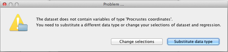
In this case, the regression analysis used Procrustes coordinates, but the dataset did not contain a data matrix with Procrustes coordinates (this can happen under somewhat spcial circumstances). In such a situation, there are two choices: click on Change selections to go back and select a different regression analysis or dataset, or click on Substitute data type for using a different data matrix in the dataset that was specified in the preceding step. If the user selects that option, choices for the data matrices and variables will need to be made manually in the next step.
After clicking Continue or Substitute data type in either of the preceding two dialog boxes, a new dialog box appears:
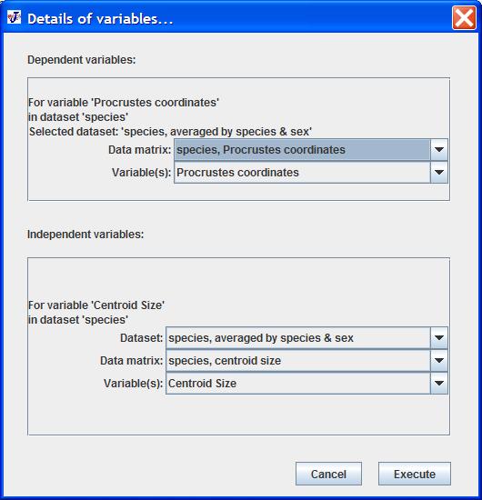
The dialog box contains elements for selecting the dependent and independent variables. MorphoJ attempts to match the variables in the selected dataset as closely as possible to those in the regression analysis. In most applications, these choices will correspond to the user's intentions, so that no changes will be needed. But there may be instances where the user wants to conduct a more complex analysis, and thus will want to make different choices.
If there was no match of the data types and variables used in the regression with the contents of the dataset, data matrices and variables need to be selected again. If there are no entries visible in a drop-down menu, click on the drop-down menu above it to reselect the item at that level, and the contents in the lower-level menu should appear.
In the top window, the choices for the dependent variables appear. As in the regression analysis in MorphoJ, all dependent variables must be from a single dataset. And because the dataset has already been chosen in the first dialog box, there is no option to change the dataset. But the data matrix (data type) and possibly individual variables can be changed.
For shape data, such as Procrustes coordinates, all shape variables are automatically selected or deselected together. Other variables, such as covariates or centroid size, can be selected individually.
The second window displays the choices for the independent variables. Here, the user can also choose a different dataset from that for the dependent variables, if this is necessary. Note that the drop-down menu only lists the datasets that are linked to the dataset with the dependent variables (see Link Datasets in the Preliminaries menu). Different independent variables can be in different datasets, but note that the same observations must be present in all datasets used in the analysis (if different observations are missing in different datasets, the final sample size can be reduced considerably).
No statistical tests are available for this procedure.
To start the analysis, click Execute. Alternatively, click Cancel to abort the procedure.
As for a regression analysis, the graphical output contains one or two panels:
If shape is used for the dependent variables, there is a graph with the shape changes corresponding to the regression vector for each independent variable. The average shape from the newly selected dataset is used as the starting shape, and the shape changes are taken directly from the regression coefficients. The default setting for this graph is the shape change for an increase of the independent variable by one unit; this can be changed by using the popup menu to alter the scale factor.
Moreover, there is a scatter plot of the regression scores (projections of the dependent variables onto the direction of the regression vector; see the explanations for regression) against the corresponding independent variable. If more than one independent variable is used, there is a plot for each of them — use the pop-up menu to switch between them.
The text output first provides information about the dependent and independent variables and the sample size.
To indicate the relative amount of variation for which the regression accounts, the output provides the total, predicted and residual sums of squares. If shape is used for the independent variables, these sums of squares are in units of squared Procrustes distance. The output also provides the proportion of variation for which the regression accounts as a percentage of the total variation. (Note: if the dependent variables are not shape, these quantities are only meaningful if all dependent variables are in the same units.)
In the context where a regression from one dataset has been applied to another dataset, these quantities are purely descriptive, and should be interpreted with caution. A regression carried out in that dataset would almost certainly produce a better fit of the data. The biological context is key to the interpretation of the results (e.g. in the comparison of variation within and between groups, as in the example used above).
The output dataset is structured in the same way as an output dataset from a regression analysis. MorphoJ generates a new dataset that contains the residuals and predicted values as well as the regression scores for every observation in the analysis.
This dataset can be used for further analyses that are the main goal of the procedure. For instance, using the residuals from a regression of shape on centroid size is a method to correct for the effects of allometry even in contexts where different datasets have to be used for estimating allometric patterns and applying them (Klingenberg and Marugán-Lobón 2013; Strelin et al. 2016).
Klingenberg, C. P. 2016. Size, shape, and form: concepts of allometry in geometric morphometrics. Development Genes and Evolution: advance online, DOI: 10.1007/s00427-00016-00539-00422.
Klingenberg, C. P., and J. Marugán-Lobón. 2013. Evolutionary covariation in geometric morphometric data: analyzing integration, modularity and allometry in a phylogenetic context. Systematic Biology 62:591–610.
Strelin, M. M., S. M. Benitez-Vieyra, J. Fornoni, C. P. Klingenberg, and A. A. Cocucci. 2016. Exploring the ontogenetic scaling hypothesis during the diversification of pollination syndromes in Caiophora (Loasaceae, subfam. Loasoideae). Annals of Botany 117:937–947.